Disgusting Code: GeoIP lookups in Excel

The challenge was to try implementing GeoIP lookups in native Excel formulas. So no HTTP calls, no macros, no add ins. This was simply to pass the time on the train but, if you’re on a very locked down machine, this will work. For example, if you’re unlucky enough to need to do log analysis on a corporate machine.

What follows is disgusting. There are a huge number of preferable ways to do Geo-IP lookups (PowerShell, macros, asking Cortana, pen and paper) but this was just some fun and is too horrific not to share.

The challenge was to write formulas that met the following constraints:

• Native formulas, no macros in case lockdown prevents macros
• Cannot call out to a website, might be blocked
• Must be position independent so can be copied to any cell on any sheet

Megamind release their geoip databases as csv files, you can import these into Excel and then use a position independent formula to search them for IP locations. This method uses formulas to convert the dotted quad form of IP addresses to decimal and then looks up the owner in the Megamind dataset.

Time to create sheet is around 5 mins and you only do it once

Time to use in a sheet for analysis is around 2 minutes.

• Goto http://dev.maxmind.com/geoip/geoip2/geolite2/ and get the Country level CSVs
• Open Excel
• Rename a sheet to “ip_lookups”
• Goto Data toolbar select “add from text” and select the “Geoip-country-blocks-IPv4.csv” you downloaded
• Rename a different sheet to “country_mapping”
• Goto data toolbar select “add from text” and select “Geoip-country-locations-en.csv”
• In “ip_lookups” sheet:
  1. Add 2 columns to the right of the IP address column (A).
  2. In cell B2 add the formula =LEFT(A2,FIND("/",A2)-1)
  3. Copy the formula to fill the whole of column B
  4. A good way to do this is to select the cell you have added the formula to and double click the bottom right corner of the cell.
  5. Add the formula below (without newlines) to the cell C2
  6. Copy formula to all other rows in column C. See above instructions for a quicker way to do it

Warning, looking at this formula may cause eye damage and a sudden affection for Lisp.

Then:

• Delete the header row (row 1)
• Sort the data on the converted numbers Column C from smallest to largest
• Save this sheet for future use

• Copy the two sheets you created previously into your workbook with logs or IP addresses
• Add a column to the right of the column that contains the IP addresses you wish to GeoIP lookup
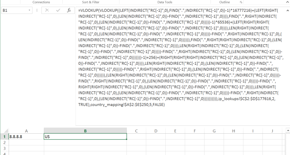
• In the column to the right, add the (dirty) formula below:

At the end of the formula, you’ll see ip_lookups!A1:C160975

• Select it, press delete and then click to your ip_lookups sheet and select all of the rows for column C and D. Shift, control and arrow keys make this easier.
  • Add $ signs to make it absolute, i.e. ip_lookups!C1:D160975 becomes ip_lookups!$C$1:$D$160975
• Go back to the end of the formula, and you’ll seecountry_mapping!A2:E249
  • Select over it, press delete and click to your “country_mapping” sheet and select over all the data as above.
  • Add $ signs to make it absolute, i.e. country_mapping!A2:E249 becomes country_mapping!$A$2:$E$249
• Drag the formula down the column to cover all of your data!

GeoIP!!!!

There are possibly going to be errors. For example it assumes all blocks are taken and are blocks are contiguous and that Megamind won’t change CSV format (this guide worked as of March 2015). If you spot any big issues or have suggested improvements (beyond ‘kill it with fire’) please let us know.